Field Effect in an MOS Structure

Numerical Experiments with Matlab

Guofu Niu

Table of Contents

1. Description

2. The main Matlab program

Graphics of Results

3. Total, Depletion and Inversion Charges

4. Common Supporting Functions

5. Beautify Your Matlab Graphics

Chapter 1. Description

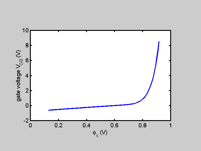
The doping concentration for the p-type body is 5.000000e+015 /cm3. The gate oxide thickness is 30 nm. The following matlab program calculates the gate voltage as a function of surface potential. The intermediate variable is the total charge density in silicon body.

Field Effect . The essence of field-effect is modulation of the inversion charge by controlling the surface potential. As we discussed in detail in our lecture, the total charges, including both inversion charges and depletion charges, can be written as a function of surface potential. The potential drop across the gate oxide is then obtained as a function of the surface potential. The sum of the potential drop across the gate oxide and across the silicon surface space charge region (equal to surface potential) gives the gate voltage. This way we obtain a curve of gate voltage versus surface potential. This method avoids solving the surface potential for a given gate voltage, which does not have an explicit solution.

Chapter 2. The main Matlab program

vgphis.m

startup;

Na = 5e15; %cm
tox_nm = 30; %nm
tox = tox_nm * 1e-7; % to cm
dum = 0;

% dielectric const of oxide
ep_ox = get_const('EpsilonOxide');

Cox = ep_ox / tox;

phi_bi = 0.56 + phi_f(Na);

% thermal voltage
p_t = get_const('ThermalVoltage');

% define the range of surface potential
% in terms of thermal voltage
ps_st = 5*p_t;
ps_en = 2*phi_f(Na) + 10*p_t;
N=100;

ps = linspace(ps_st, ps_en, N);

Q_s = qs(ps, Na);

phi_g = ps + Q_s./Cox;

Vg = phi_g - phi_bi;

figure(1);

plot(ps, Vg);
xlabel('\phi_s (V)');
ylabel('gate voltage V_{GB} (V)');

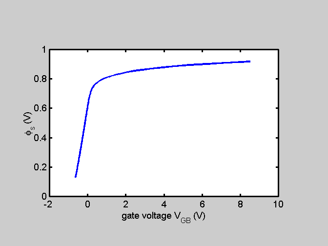
figure(2);
plot(Vg, ps);
ylabel('\phi_s (V)');
xlabel('gate voltage V_{GB} (V)');

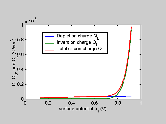
figure(3);
Q_b = qb(ps, Na);
Q_i = qinv(ps, Na);
plot(ps, Q_b, ps, Q_i, ps, Q_s);
xlabel('surface potential \phi_s (V)');
ylabel('Q_I, Q_B, and Q_S (C/cm^2)');
legend('Depletion charge Q_B', 'Inversion charge Q_I', 'Total silicon charge Q_S');

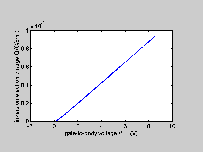
figure(4);
plot(Vg, Q_i);
xlabel('gate-to-body voltage V_{GB} (V)');
ylabel('inversion electron charge Q_I (C/cm^2)');

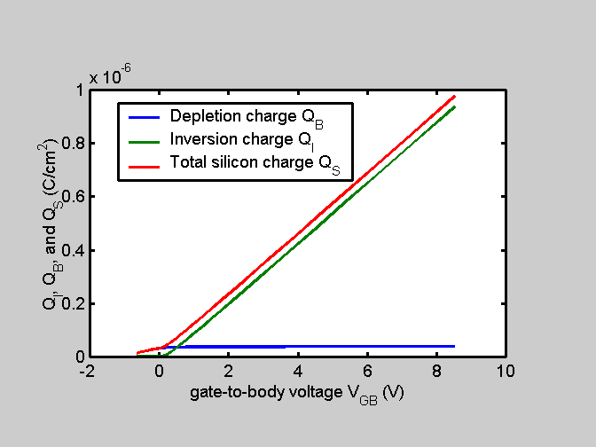
figure(5);
plot(Vg, Q_b, Vg, Q_i, Vg, Q_s);
xlabel('gate-to-body voltage V_{GB} (V)');
ylabel('Q_I, Q_B, and Q_S (C/cm^2)');
legend('Depletion charge Q_B', 'Inversion charge Q_I', 'Total silicon charge Q_S');

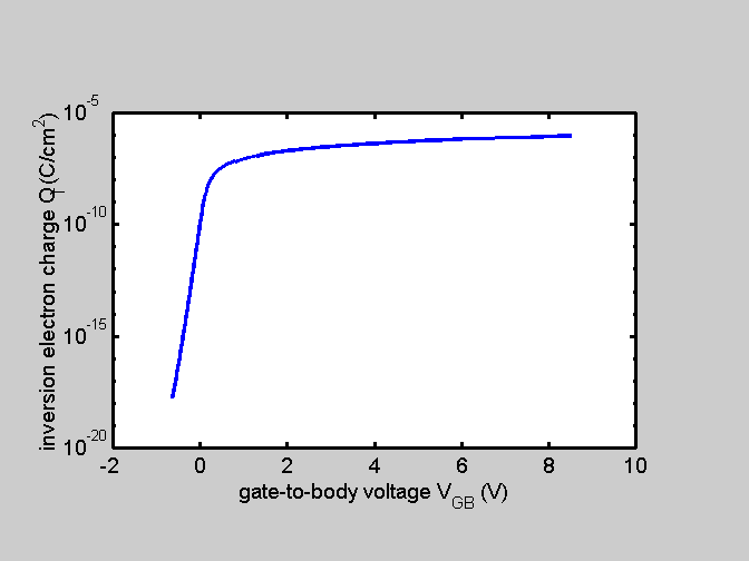
figure(6);
semilogy(Vg, Q_i);
xlabel('gate-to-body voltage V_{GB} (V)');
ylabel('inversion electron charge Q_I (C/cm^2)');

Graphics of Results

Chapter 3. Total, Depletion and Inversion Charges

Total charge in silicon body Qs . The following is the matlab code for Qs. The input parameters are surface potential phi_s, and doping concentration Na.

qs.m

function qs = qs(phi_s, Na)
dum = 0;
p_t = get_const('ThermalVoltage');
p_f = phi_f(Na);
tmp1 = get_const('sqrt_2qeps');
tmp2 = sqrt(Na);
tmp3 = (phi_s - 2*p_f)./p_t;
tmp4 = sqrt(phi_s + p_t.*exp(tmp3));
qs = tmp1*tmp2*tmp4;

Depletion charge in Si body Qb . The following program calculates Qb, the depletion charge, as a function of phi_s, the surface potential, and Na.

qb.m

function qb = qb(phi_s, Na)
% qb - returns area depletion charge
% phi_s: surface potential (in V)
% Na: p-type body doping (in /cm^3)
tmp1 = get_const('sqrt_2qeps');
tmp2 = sqrt(Na);
tmp4 = sqrt(phi_s);
qb = tmp1*tmp2*tmp4;

Inversion Charge QI (electron charge) . Inversion charge QI is simply the difference between the total silicon charge and the silicon depletion charge.

qinv.m

function qi = qinv(phi_s, Na)
qi = qs(phi_s, Na) - qb(phi_s, Na);

Chapter 4. Common Supporting Functions

Physical Constants . The following introduces how to use the function get_const(constantName) to get values of physical constants. I wrote this function to allow you easily add your own constant definition by modifying get_const.m. These are handy when you need to write some program related to field-effect transistor operation and modeling.

Usage

For example, to get the value of a constant like thermal voltage is easy, simply use:

phi_t = get_const('ThermalVoltage');

or:

phi_t = get_const('phi_t');

or

phi_t = get_const('Vt');

or

phi_g = get_const('V_t');

For the value of intrinsic concentration:

ni = get_const('ni');

or

ni = get_const('IntrinsicConcentration');

Physical Constants Related to MOSFET get_const.m

function answer = get_const(constName)
% get_const: returns value of a physical constant
%
switch lower(constName)
  case {'phi_t', 'thermalvoltage', 'vt', 'v_t'}
     answer = 25.8e-3; % V
  case {'eps_si', 'epssi', 'epssilicon','epsilonsilicon'}
     answer = 1.04e-12; % F/cm
  case {'eps_ox', 'epsilonoxide', 'epsox', 'epssio2', 'epsoxide'}
     answer = 3.45e-13; % F/cm
  case {'ni', 'intrinsicn', 'n_i', 'intrinsicconcentration', 'intrinsicconc'}
     answer = 1.4e10; % /cm^3
  case {'q', 'echarge', 'elementarycharge','electroncharge'}
     answer = 1.602e-19; % C
  case {'sqrt_2qeps','sqrt2qeps'}
     answer = 5.79e-16; % FV^(1/2)cm^(-1/2)
  otherwise
     display('Unknown constant name');
end

Fermi Potential phi_f.m

function phi = phi_f(Na)
% phi_f - returns Fermi potential of p-type body
% Na - doping conc in /cm^3
dum = 0;
p_t = get_const('ThermalVoltage');
n_i = get_const('IntrinsicConcentration');
phi = p_t .* log(Na/n_i);

Chapter 5. Beautify Your Matlab Graphics

Graphics Setting . Default matlab graphics may not be satisfactory. Lines are too thin, and fonts are too small. This is often a problem if you need to include a matlab figure in your report or paper. If you are using UNIX, put this following startup.m file in your working directory, and then start matlab from your working directory. If you are using windows, you can simply put the following statement as your first matlab statement: startup; ....

% start up file startup.m
% change the font size and line width as well as axes position

set(0,'DefaultAxesFontSize',12);
set(0,'DefaultTextFontSize',12);
set(0,'DefaultAxesLinewidth',2);
set(0,'DefaultLineLinewidth',2);
set(0,'DefaultAxesPosition',[0.15 0.2 0.7 0.6]);